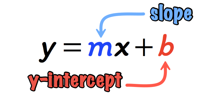
The slope-intercept is the most “popular” form of a straight line. Many students find this useful because of its simplicity. One can easily describe the characteristics of the straight line even without seeing its graph because the slope and [latex]y[/latex]-intercept can easily be identified or read off from this form.
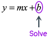
The linear equation written in the form
is in slope-intercept form where:
[latex]m[/latex] is the slope, and [latex]b[/latex] is the [latex]y[/latex]-intercept

Quick notes:
Let’s go over some examples of how to write the equation of a straight line in linear form [latex]y = mx + b[/latex].
Example 1: Write the equation of the line in slope-intercept form with a slope of [latex] – \,5[/latex] and a [latex]y[/latex]-intercept of [latex]3[/latex].
The needed information to write the equation of the line in the form [latex]y = mx + b[/latex] are clearly given in the problem since
[latex]m = – \,5[/latex] (slope)
[latex]b = 3[/latex] ([latex]y[/latex]-intercept)
Substituting in [latex]y = mx + b[/latex], we obtain
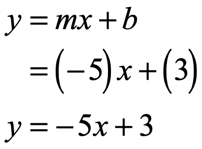
By having a negative slope, the line is decreasing/falling from left to right, and passing through the [latex]y[/latex]-axis at point [latex]\left( \right)[/latex].
Example 2: Write the equation of the line in slope-intercept form with a slope of [latex]7[/latex] and a [latex]y[/latex]-intercept of [latex] – \,4[/latex].
The slope is given as [latex]m = 7[/latex] and the [latex]y[/latex]-intercept as [latex]b = – \,4[/latex]. Substituting into the slope-intercept formula [latex]y = mx + b[/latex], we have
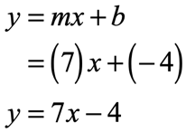
The slope is positive thus the line is increasing or rising from left to right, but passing through the [latex]y[/latex]-axis at point [latex]\left( \right)[/latex].
Example 3: Write the equation of the line in slope-intercept with a slope of [latex]9[/latex] and passing through the point [latex]\left( \right)[/latex].
This problem is slightly different from the previous two examples because the [latex]y[/latex]-intercept [latex]b[/latex] is not given to us upfront. So our next goal is to somehow figure out the value of [latex]b[/latex] first.
However, if we examine the slope-intercept form, it should lead us to believe that we have enough information to solve for [latex]b[/latex]. How?
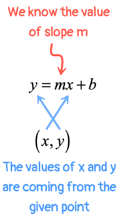
That means [latex]m = 9[/latex], and from the given point [latex]\left( \right)[/latex] we have [latex]x = 0[/latex] and [latex]y = – \,2[/latex]. Let’s substitute these known values into the slope-intercept formula and solve for the missing value of [latex]b[/latex].
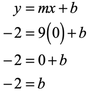
Now it is possible to write the slope-intercept form as
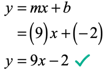
Example 4: Find the slope-intercept form of the line with a slope of [latex] – \,3[/latex] and passing through the point [latex]\left( < – 1,\,15>\right)[/latex].
Again, the value of [latex]y[/latex]-intercept [latex]b[/latex] is not directly provided to us. But we can utilize the given slope and a point to find it.
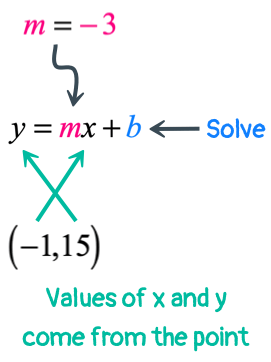
Substitute the known values into the slope-intercept formula, and then solve for the unknown value of [latex]b[/latex].
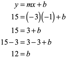
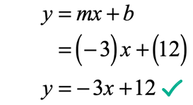
Back substitute the value of the slope and the solved value of the [latex]y[/latex]-intercept into [latex]y = mx + b[/latex].
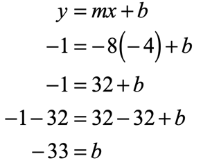
Example 5: A line with the slope of [latex] – \,8[/latex] and passing through the point [latex]\left( < – \,4,\, – 1>\right)[/latex].
The given slope is [latex]m = – \,8[/latex] and from the given point [latex]\left( < – \,4,\, – 1>\right)[/latex], we have [latex]x = – \,4[/latex] and [latex]y = – \,1[/latex]. Now, we are going to substitute the known values into the slope-intercept form of the line to solve for [latex]b[/latex].
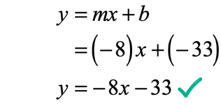
Since [latex]m = – \,8[/latex] and [latex]b = – \,33[/latex], the slope-intercept form of the line becomes
Example 6: Write the slope-intercept form of the line with a slope of [latex][/latex] and through the point [latex]\left( \right)[/latex].
We have a slope here that is not an integer, i.e. the denominator is other than positive or negative one, [latex] \pm 1[/latex]. In other words, we have a “true” fractional slope.
The procedure for solving this problem is very similar to examples #3, #4, and #5. But the main point of this example is to emphasize the algebraic steps required on how to solve a linear equation involving fractions.
The known values of the problem are
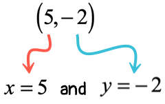
Plug the values into [latex]y = mx + b[/latex] and solve for [latex]b[/latex].
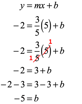
As you can see the common factors of [latex]5[/latex] in the numerator and denominator nicely cancel each other out which greatly simplifies the process of solving for [latex]b[/latex].
Putting this together in the form [latex]y = mx + b[/latex]
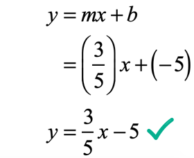
Example 7: Slope of [latex] \over 2>[/latex] and through the point [latex]\left( < – 1,\, – 1>\right)[/latex].
The given slope is [latex]m = \over 2>[/latex] and from the given point [latex]\left( < – 1,\, – 1>\right)[/latex], the values of [latex]x[/latex] and [latex]y[/latex] can easily be identified.
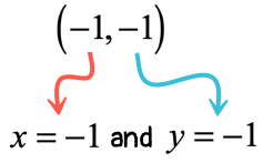
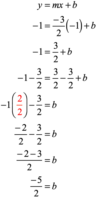
Now plug in the known values into the slope-intercept form [latex]y = mx + b[/latex] to solve for [latex]b[/latex].
Make sure that when you add or subtract fractions, you generate a common denominator.
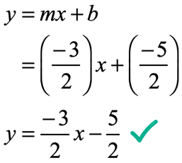
After getting the value of [latex]b[/latex], we can now write the slope-intercept form of the line.
Example 8: Slope of [latex] – \,6[/latex] and through the point [latex]\left( ,> \right)[/latex].
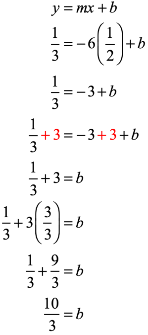
The slope is given as [latex]m = – \,6[/latex] and from the point, we have [latex]x = [/latex] and [latex]y = [/latex].
Substitute the known values into [latex]y = mx + b[/latex]. Then solve the missing value of [latex]b[/latex] .
Therefore, the slope-intercept form of the line is
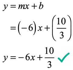
Example 9: Slope of [latex] \over 3>[/latex] and through the point [latex]\left( \over 5>,> \right)[/latex].
Identifying the known values
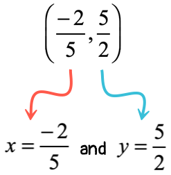
The setup to find [latex]b[/latex] becomes
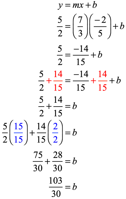
That makes the slope-intercept form of the line as
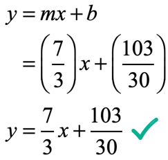
Example 10: A line passing through the given two points [latex]\left( \right)[/latex] and [latex]\left( \right)[/latex].
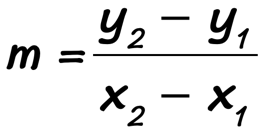
In this problem, we are not provided with both the slope [latex]m[/latex] and [latex]y[/latex]-intercept [latex]b[/latex]. However, we should realize that the slope is easily calculated when two points are known using the Slope Formula.
The slope, [latex]m[/latex], of a line passing through two arbitrary points [latex]\left( ,> \right)[/latex] and [latex]\left( ,> \right)[/latex] is calculated as follows…

If we let [latex]\left( \right)[/latex] be the first point, then [latex]\left( \right)[/latex] must be the second.
Labeling the components of each point should help in identifying the correct values that would be substituted into the slope formula.
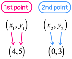 has the x-coordinate of 4 and a y-coordinate of 5 while the second ordered pair (x2,y2) has the x-coordinate of 0 and a y-coordinate of 3." width="282" height="234" />
Based on the labeling above, now we know that

Next, write the slope formula, plug in the known values and simplify.
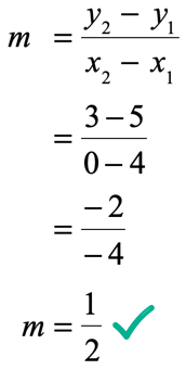
Great! We found the slope to be [latex]m = \over 2>\,[/latex]. The only missing piece of the puzzle is to determine the [latex]y[/latex]-intercept. Use the slope that we found, together with ANY of the two given points. In this exercise, I will show you that we should arrive at the same value of the [latex]y[/latex]-intercept regardless of which point is selected for the calculation.
Finding the [latex]y[/latex]-intercept
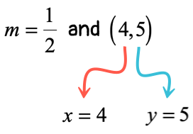
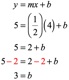
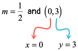
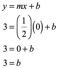
Indeed, the [latex]y[/latex]-intercepts come out the same in both calculations. We can now write the linear equation in slope-intercept form.
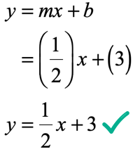
Below is the graph of the line passing through the given two points.
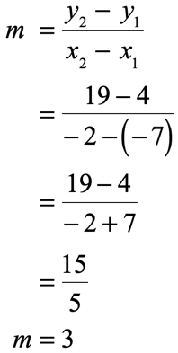
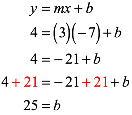
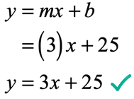
Example 11: A line passing through the given two points [latex]\left( < – \,7,\,4>\right)[/latex] and [latex]\left( < – \,2,\,19>\right)[/latex].
Let’s solve this step by step.
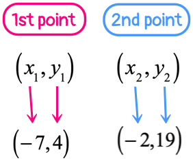
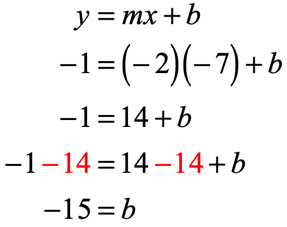
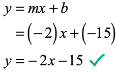
Example 12: A line passing through the given two points [latex]\left( < – \,6,\, – \,3>\right)[/latex] and [latex]\left( < – \,7,\, – 1>\right)[/latex].
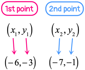
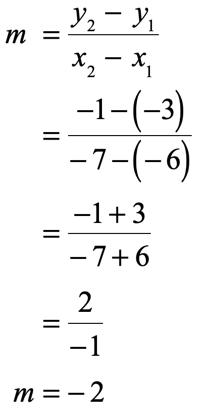
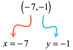
Substitute known values in the slope-intercept form [latex]y = mx + b[/latex] to solve for [latex]b[/latex].
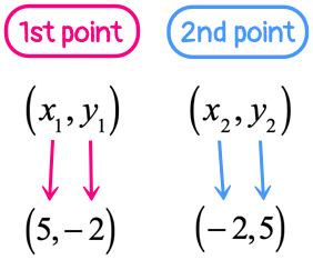
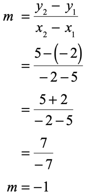
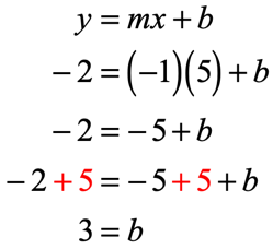
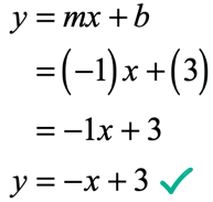
Example 13: A line passing through the given two points [latex]\left( \right)[/latex] and [latex]\left( < – \,2,\,5>\right)[/latex].
You might also like these tutorials:
Categories